Example of a linar chirp waveform

1. Instantiate the waveform

from pathlib import Path
import os
from tfwaves import waveform, stft, response
import numpy as np
from matplotlib import pyplot as plt
from matplotlib import colors
import urllib, os
from scipy.signal import ShortTimeFFT

# Look at one month of data
tobs = 30 * 24 * 3600
# Sampling rate
fs = 1 / 10.0  # 10 second sampling rate
# Initial frequency in Hz
f0 = 1.0e-3 # 0.5e-3  
# Initial frequency derivative in Hz/s
fdot0 = 1e-9
# Frequency at the end of the observation period
f_end = f0 + fdot0 * tobs
print(f"End frequency after {tobs/(24*3600):.1f} days is {f_end*1e3:.3f} mHz")
# Comparison with Nyquist frequency
f_nyquist = fs / 2
print(f"Nyquist frequency is {f_nyquist*1e3:.3f} mHz")
# Create linear chirp waveform
linear_chirp = waveform.LinearChirp(f0=f0,  fdot0=fdot0)

End frequency after 30.0 days is 3.592 mHz
Nyquist frequency is 50.000 mHz

# Create a time vector with 10 second sampling rate
t_grid = np.arange(0, tobs, 1 / fs)
# Compute the strain
h = linear_chirp.compute_strain(t_grid)

# Plot the plus and cross components as a function of time
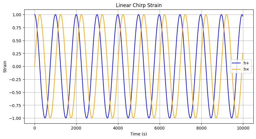
plt.figure(figsize=(10, 5))
plt.plot(t_grid[0:1000], h.real[0:1000], label='h+', color='blue')
plt.plot(t_grid[0:1000], -h.imag[0:1000], label='h×', color='orange')
plt.xlabel('Time (s)')
plt.ylabel('Strain')
plt.title('Linear Chirp Strain')
plt.legend()
plt.grid()
plt.show()

2. Compute its STFT from the time series

# # The URL for the orbit data
# orbits_url = "https://lisa-ldc.in2p3.fr/media/uploads/orbits.h5"
# if not os.path.exists("orbits.h5"):
#     urllib.request.urlretrieve(orbits_url, "orbits.h5")

# Choose the duration of one time window
window_duration = 24 * 3600 # 6 * 3600 # 24 * 3600  # seconds
# Size of the time window in samples
window_size = int(window_duration * fs)  # 10 second sampling rate
# Window function
w = np.ones(window_size)
# Orbits
orbit_path = Path(os.getcwd()).resolve().parents[1] / "tests" / "orbits.h5"
# Starting time of observation
t_start = 30 * 24 * 3600  # 30 days
# Set source configuration
config = stft.ObservationConfig(
    orbit_path=orbit_path,
    t_start=t_start,
    size=len(t_grid),
)
# Create the STFT object
stft_obj = stft.TimeToTFWaveform(
    w,
    window_size,
    fs,
    waveform=linear_chirp,
    config=config,
)
# Compute the STFT of the waveform
scp_stft = ShortTimeFFT(w, hop=window_size, fs=fs, mfft=None, scale_to='magnitude')
s_plus = scp_stft.stft(h.real)
s_cross = scp_stft.stft(-h.imag)

You are using an orbit file in a version that might not be fully supported

# Compute the waveform frequency at the time grid
f_time = linear_chirp.compute_frequencies(t_grid)
# Compute the waveform frequency derivative at the time grid
df_time = linear_chirp.compute_frequencies_derivatives(t_grid)

N = h.size  # number of samples in the time series
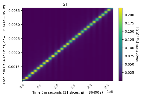
fig1, ax1 = plt.subplots(figsize=(6., 4.))  # enlarge plot a bit
t_lo, t_hi = scp_stft.extent(N)[:2]  # time range of plot
ax1.set_title(rf"STFT")
ax1.set(xlabel=f"Time $t$ in seconds ({scp_stft.p_num(N)} slices, " +
               rf"$\Delta t = {scp_stft.delta_t:g}\,$s)",
        ylabel=f"Freq. $f$ in Hz ({scp_stft.f_pts} bins, " +
               rf"$\Delta f = {scp_stft.delta_f:g}\,$Hz)",
        xlim=(t_lo, t_hi))
ax1.set_ylim([f_time[10], f_time[-10]])
im1 = ax1.imshow(abs(s_plus), origin='lower', aspect='auto',
                 extent=scp_stft.extent(N), cmap='viridis')
# ax1.plot(t_x, f_i, 'r--', alpha=.5, label='$f_i(t)$')
fig1.colorbar(im1, label=r"Magnitude $|S_{h+}(t, f)|$")
fig1.tight_layout()
plt.tick_params(axis='x', rotation=45)
plt.show()

3. Compute its STFT analytically

# STFT time bins
t_bins = np.arange(s_plus.shape[1]) * stft_obj.delta_t 
# What should be the margin around f(t) ? Use the variation of frequency within one time bin
margin = np.max(df_time * stft_obj.delta_t / stft_obj.delta_f)
di = 2*round(margin)
s_plus_approx, s_cross_approx, indices_f, indices_t = stft_obj.compute_hphc(di=di)
# Convert to dense arrays
s_plus_approx_dense = s_plus_approx.toarray()
s_cross_approx_dense = s_cross_approx.toarray()

---------------------------------------------------------------------------
AttributeError                            Traceback (most recent call last)
Cell In[8], line 8
      4 margin = np.max(df_time * stft_obj.delta_t / stft_obj.delta_f)
      5 di = 2*round(margin)
      6 s_plus_approx, s_cross_approx, indices_f, indices_t = stft_obj.compute_hphc(di=di)
      7 # Convert to dense arrays
----> 8 s_plus_approx_dense = s_plus_approx.toarray()
      9 s_cross_approx_dense = s_cross_approx.toarray()

AttributeError: 'numpy.ndarray' object has no attribute 'toarray'

N = h.size  # number of samples in the time series
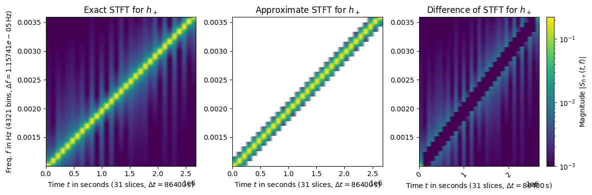
fig1, ax1 = plt.subplots(nrows=1, ncols=3, figsize=(12., 4.))  # enlarge plot a bit
t_lo, t_hi = scp_stft.extent(N)[:2]  # time range of plot

# Use a logarithmic color scale
norm = colors.LogNorm(vmin=1e-3, vmax=abs(s_plus).max())

# TRUE
ax1[0].set_title(rf"Exact STFT for $h_+$")
ax1[0].set(xlabel=f"Time $t$ in seconds ({scp_stft.p_num(N)} slices, " +
               rf"$\Delta t = {scp_stft.delta_t:g}\,$s)",
        ylabel=f"Freq. $f$ in Hz ({scp_stft.f_pts} bins, " +
               rf"$\Delta f = {scp_stft.delta_f:g}\,$Hz)",
        xlim=(t_lo, t_hi))
ax1[0].set_ylim([f_time[10], f_time[-10]])
im0 = ax1[0].imshow(abs(s_plus), origin='lower', aspect='auto',
                 extent=scp_stft.extent(N), cmap='viridis', norm=norm)


# APPROXIMATE
ax1[1].set_title(rf"Approximate STFT for $h_+$")
ax1[1].set(xlabel=f"Time $t$ in seconds ({scp_stft.p_num(N)} slices, " +
               rf"$\Delta t = {scp_stft.delta_t:g}\,$s)",
        xlim=(t_lo, t_hi))
ax1[1].set_ylim([f_time[10], f_time[-10]])
im1 = ax1[1].imshow(abs(s_plus_approx_dense), origin='lower', aspect='auto',
                 extent=scp_stft.extent(N), cmap='viridis', norm=norm)


# DIFFERENCE
ax1[2].set_title(rf"Difference of STFT for $h_+$")
ax1[2].set(xlabel=f"Time $t$ in seconds ({scp_stft.p_num(N)} slices, " +
               rf"$\Delta t = {scp_stft.delta_t:g}\,$s)",
        xlim=(t_lo, t_hi))
ax1[2].set_ylim([f_time[10], f_time[-10]])
im2 = ax1[2].imshow(abs(s_plus_approx_dense - s_plus), origin='lower', aspect='auto',
                 extent=scp_stft.extent(N), cmap='viridis', norm=norm)


fig1.colorbar(im2, label=r"Magnitude $|S_{h+}(t, f)|$")
fig1.tight_layout()
plt.tick_params(axis='x', rotation=45)
plt.show()

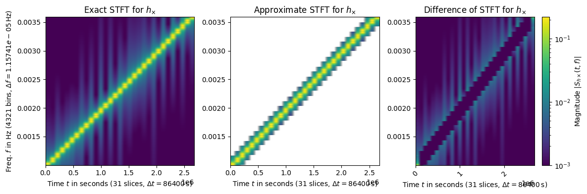
N = h.size  # number of samples in the time series
fig1, ax1 = plt.subplots(nrows=1, ncols=3, figsize=(12., 4.))  # enlarge plot a bit
t_lo, t_hi = scp_stft.extent(N)[:2]  # time range of plot

# Use a logarithmic color scale
norm = colors.LogNorm(vmin=1e-3, vmax=abs(s_cross).max())

# TRUE
ax1[0].set_title(r"Exact STFT for $h_{\times}$")
ax1[0].set(xlabel=f"Time $t$ in seconds ({scp_stft.p_num(N)} slices, " +
               rf"$\Delta t = {scp_stft.delta_t:g}\,$s)",
        ylabel=f"Freq. $f$ in Hz ({scp_stft.f_pts} bins, " +
               rf"$\Delta f = {scp_stft.delta_f:g}\,$Hz)",
        xlim=(t_lo, t_hi))
ax1[0].set_ylim([f_time[10], f_time[-10]])
im0 = ax1[0].imshow(abs(s_cross), origin='lower', aspect='auto',
                 extent=scp_stft.extent(N), cmap='viridis', norm=norm)


# APPROXIMATE
ax1[1].set_title(r"Approximate STFT for $h_{\times}$")
ax1[1].set(xlabel=f"Time $t$ in seconds ({scp_stft.p_num(N)} slices, " +
               rf"$\Delta t = {scp_stft.delta_t:g}\,$s)",
        xlim=(t_lo, t_hi))
ax1[1].set_ylim([f_time[10], f_time[-10]])
im1 = ax1[1].imshow(abs(s_cross_approx_dense), origin='lower', aspect='auto',
                 extent=scp_stft.extent(N), cmap='viridis', norm=norm)

# DIFFERENCE
ax1[2].set_title(r"Difference of STFT for $h_{\times}$")
ax1[2].set(xlabel=f"Time $t$ in seconds ({scp_stft.p_num(N)} slices, " +
               rf"$\Delta t = {scp_stft.delta_t:g}\,$s)",
        xlim=(t_lo, t_hi))
ax1[2].set_ylim([f_time[10], f_time[-10]])
im2 = ax1[2].imshow(abs(s_cross_approx_dense - s_cross), origin='lower', aspect='auto',
                 extent=scp_stft.extent(N), cmap='viridis', norm=norm)


fig1.colorbar(im2, label=r"Magnitude $|S_{h\times}(t, f)|$")
fig1.tight_layout()
plt.tick_params(axis='x', rotation=45)
plt.show()

# Error as a function of time
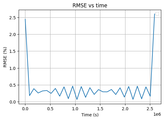
squared_error = abs(s_cross_approx_dense - s_cross)**2
rmse_vs_time = np.mean(squared_error, axis=0)
# RMSE in percent of amplitude
rmse_vs_time = np.sqrt(rmse_vs_time) / np.max(abs(s_cross), axis=0) * 100

plt.figure(figsize=(6, 4))
plt.plot(t_bins, rmse_vs_time)
plt.xlabel('Time (s)')
plt.ylabel('RMSE (%)')
plt.title('RMSE vs time')
plt.legend()
plt.grid()
plt.show()

/var/folders/j3/bxsfgp354m71s36hk2dpg4p80000gn/T/ipykernel_94761/611977175.py:6: UserWarning: No artists with labels found to put in legend.  Note that artists whose label start with an underscore are ignored when legend() is called with no argument.
  plt.legend()

# Evaluate the normalized RMSE on the track
rmse = np.sqrt(np.mean(abs(s_plus_approx_dense[:, 1:-1] - s_plus[:, 1:-1])**2))
print("RMSE for h+:", rmse)

RMSE for h+: 0.0006505908684125557

# Evaluate the normalized RMSE on the track
rmse = np.sqrt(np.mean(abs(s_cross_approx_dense[:, 1:-1] - s_cross[:, 1:-1])**2))
print("RMSE for hx:", rmse)

RMSE for hx: 0.0006500222284841215

4. Compute arm responses

4.1 Exact responses

dec=0.0
ra=0.0

# Compute response with LISA ring
response_lisaring = response.ResponseFromStrain(
            orbits=orbit_path,
            dt=1/fs,  # This is the coarse grid
            # Should it be the STFT time resolution?
            size=len(t_grid),  # Size of the coarse grid
            t0=stft_obj._response.t0,  # Your standard offset, should not be hard-coded
        )

You are using an orbit file in a version that might not be fully supported

response_lisaring.set_position(dec, ra)
arm_responses = response_lisaring.read_gw_response(h.real, -h.imag, stft_obj._response.t0 + t_grid,
                                                   strain_interp_order=5, dictt=False).T
s_links_exact = np.asarray([scp_stft.stft(arm_responses[:, i]) for i in range(6)])
s_links_exact = np.swapaxes(s_links_exact, 1, 2).T

4.2 Approximate responses

stft_obj._build_response(dec, ra)
s_links_approx, indices_f, indices_t = stft_obj.compute_arm_response_tf(di=di)
# Convert to full array
s_links_approx_full = np.zeros_like(s_links_exact)
s_links_approx_full[indices_f, indices_t, :] = s_links_approx

4.3 Comparison

j_link = 0
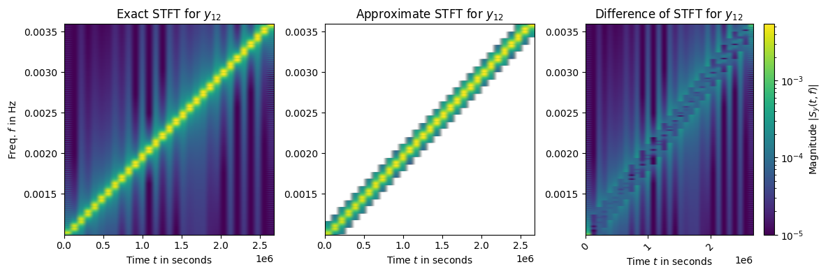
fig1, ax1 = plt.subplots(nrows=1, ncols=3, figsize=(12., 4.))  # enlarge plot a bit

# Logarithmic color scale
norm = colors.LogNorm(vmin=1e-5,
                      vmax=abs(s_links_exact[..., j_link]).max())

# TRUE
ax1[0].set_title(r"Exact STFT for $y_{12}$")
ax1[0].set(xlabel=r"Time $t$ in seconds",
           ylabel=r"Freq. $f$ in Hz",
        xlim=(t_lo, t_hi))
ax1[0].set_ylim([f_time[10], f_time[-10]])
im0 = ax1[0].imshow(abs(s_links_exact[..., j_link]), origin='lower', aspect='auto',
                    extent=scp_stft.extent(N), cmap='viridis', norm=norm)

# APPROXIMATE
ax1[1].set_title(r"Approximate STFT for $y_{12}$")
ax1[1].set(xlabel=r"Time $t$ in seconds",
        xlim=(t_lo, t_hi))
ax1[1].set_ylim([f_time[10], f_time[-10]])
im1 = ax1[1].imshow(abs(s_links_approx_full[..., j_link]), origin='lower', aspect='auto',
                 extent=scp_stft.extent(N), cmap='viridis', norm=norm)
# ax1.plot(t_x, f_i, 'r--', alpha=.5, label='$f_i(t)$')


# DIFFERENCE
ax1[2].set_title(r"Difference of STFT for $y_{12}$")
ax1[2].set(xlabel=r"Time $t$ in seconds",
        xlim=(t_lo, t_hi))
ax1[2].set_ylim([f_time[10], f_time[-10]])
im2 = ax1[2].imshow(abs(s_links_approx_full[..., j_link] - s_links_exact[..., j_link]), 
                    origin='lower', aspect='auto',
                    extent=scp_stft.extent(N), cmap='viridis', norm=norm)


fig1.colorbar(im2, label=r"Magnitude $|S_{y}(t, f)|$")
fig1.tight_layout()
plt.tick_params(axis='x', rotation=45)
plt.show()

# Error as a function of time
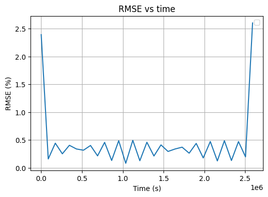
squared_error = abs(s_links_approx_full[..., j_link] - s_links_exact[..., j_link])**2
rmse_vs_time = np.mean(squared_error, axis=0)
# RMSE in percent of amplitude
rmse_vs_time = np.sqrt(rmse_vs_time) / np.max(abs(s_links_exact[..., j_link]), axis=0) * 100

print(np.max(rmse_vs_time[1:-1]))

0.4926503962682829

plt.figure(figsize=(6, 4))
plt.plot(t_bins, rmse_vs_time)
plt.xlabel('Time (s)')
plt.ylabel('RMSE (%)')
plt.title('RMSE vs time')
plt.legend()
plt.grid()
plt.show()

/var/folders/j3/bxsfgp354m71s36hk2dpg4p80000gn/T/ipykernel_94761/611977175.py:6: UserWarning: No artists with labels found to put in legend.  Note that artists whose label start with an underscore are ignored when legend() is called with no argument.
  plt.legend()

5. Compute TDI responses

5.1 Exact responses

# Compute TDI with response.py
tdi_lisaring = response_lisaring.compute_tdi(h.real, -h.imag, channel="XYZ")
s_tdi1_lisaring = -np.asarray([scp_stft.stft(tdi_lisaring[key]) for key in ["TDIX", "TDIY", "TDIZ"]])
s_tdi1_lisaring = np.swapaxes(s_tdi1_lisaring, 1, 2).T

5.2 Approximate responses

s_tdi1_approx, indices_f, indices_t = stft_obj.compute_tdi_tf_response(channel="XYZ", gen="1.5", di=di)
# Convert to full array
s_tdi1_approx_full = np.zeros_like(s_tdi1_lisaring)
s_tdi1_approx_full[indices_f, indices_t, :] = s_tdi1_approx

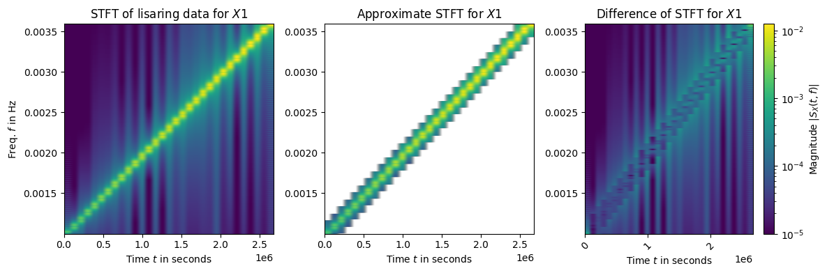
5.3 Comparison

fig1, ax1 = plt.subplots(nrows=1, ncols=3, figsize=(12., 4.))  # enlarge plot a bit

# Logarithmic color scale
norm = colors.LogNorm(vmin=1e-5,
                      vmax=abs(s_tdi1_lisaring[..., 0]).max())

# TRUE
ax1[0].set_title(r"STFT of lisaring data for $X1$")
ax1[0].set(xlabel=r"Time $t$ in seconds",
           ylabel=r"Freq. $f$ in Hz",
        xlim=(t_lo, t_hi))
ax1[0].set_ylim([f_time[10], f_time[-10]])
im0 = ax1[0].imshow(abs(s_tdi1_lisaring[..., 0]), origin='lower', aspect='auto',
                 extent=scp_stft.extent(N), cmap='viridis', norm=norm)

# APPROXIMATE
ax1[1].set_title(r"Approximate STFT for $X1$")
ax1[1].set(xlabel=r"Time $t$ in seconds",
        xlim=(t_lo, t_hi))
ax1[1].set_ylim([f_time[10], f_time[-10]])
im1 = ax1[1].imshow(abs(s_tdi1_approx_full[..., 0]), origin='lower', aspect='auto',
                 extent=scp_stft.extent(N), cmap='viridis', norm=norm)
# ax1.plot(t_x, f_i, 'r--', alpha=.5, label='$f_i(t)$')


# DIFFERENCE
ax1[2].set_title(r"Difference of STFT for $X1$")
ax1[2].set(xlabel=r"Time $t$ in seconds",
        xlim=(t_lo, t_hi))
ax1[2].set_ylim([f_time[10], f_time[-10]])
im2 = ax1[2].imshow(abs(s_tdi1_approx_full[..., 0] - s_tdi1_lisaring[..., 0]), origin='lower', aspect='auto',
                 extent=scp_stft.extent(N), cmap='viridis', norm=norm)


fig1.colorbar(im2, label=r"Magnitude $|S_{X}(t, f)|$")
fig1.tight_layout()
plt.tick_params(axis='x', rotation=45)
plt.show()

# Error as a function of time for TDI1
squared_error = abs(s_tdi1_approx_full[indices_f, :, 0] - s_tdi1_lisaring[indices_f, :, 0])**2
rmse_vs_time = np.mean(squared_error, axis=0)
# RMSE in percent of amplitude
rmse_vs_time = np.sqrt(rmse_vs_time) / np.max(abs(s_tdi1_lisaring[indices_f, :, 0]), axis=0) * 100

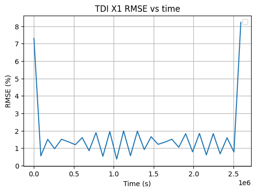
print("Max RMSE on link", j_link, ":", rmse_vs_time[1:-1].max(), "%")

Max RMSE on link 0 : 1.9879807781281085 %

plt.figure(figsize=(6, 4))
plt.plot(t_bins, rmse_vs_time)
plt.xlabel('Time (s)')
plt.ylabel('RMSE (%)')
plt.title('TDI X1 RMSE vs time')
plt.legend()
plt.grid()
plt.show()

/var/folders/j3/bxsfgp354m71s36hk2dpg4p80000gn/T/ipykernel_94761/2372180008.py:6: UserWarning: No artists with labels found to put in legend.  Note that artists whose label start with an underscore are ignored when legend() is called with no argument.
  plt.legend()